Features
Environmental Control
Heating
Lighting
Vegetables
Ventilation
Predicting the greenhouse microclimate
Gaining control of the greenhouse climate isn’t as simple as deciding on minimum and maximum setpoints.
October 13, 2020 By Quade Digweed
 Figure 2. Big leaf model (left) and density function approach (right). Image credit: AAFC
 One of the most well-known benefits of controlled environment agriculture is in the name – the control, manipulation, and optimization of the growing environment. Good control, however, is dependent on more than keeping the greenhouse air temperature and humidity between set minimum and maximum values.
If we define the greenhouse climate as the ‘macroclimate,’ then the immediate climate surrounding the crop is known as the plant ‘microclimate.’ Think of the microclimate as a bubble around the plant, a blanket of still air surrounding it. This microclimate can vary across the greenhouse and is strongly influenced by crop structure (geometry) and greenhouse management.
Uniform control of the greenhouse macroclimate does not guarantee a uniform microclimate. By predicting this variation in the canopy and the impact of control variables (e.g. temperature, humidity) on the microclimate, we can identify areas that may be prone to disease, better predict yield, and understand the influence of new technologies on the microclimate before they’re installed. Past work at the Harrow Research and Development Centre in Ontario focused on modeling the microclimate in greenhouse cucumber, while current work at Harrow is now focused on the impact of supplemental lighting on the greenhouse microclimate, specifically in greenhouse peppers. A model to predict these effects is currently under development, along with new measurement methods and technologies to directly observe the impact of lighting on the greenhouse microclimate.
Why modelling?
Just as air temperatures can vary across a greenhouse, the plant microclimate is heavily impacted by plant structure, varying between plants and vertically within the crop. While the greenhouse microclimate could be directly measured with enough sensors, the cost of measuring essential greenhouse microclimate variables (e.g. leaf and fruit temperature, wetness, light transmission, vapour pressure deficit, CO2) at the density required for meaningful predictions would be prohibitive for most growers. By first developing a model in a research greenhouse equipped with the required sensors, predictions can be made and applied to commercial production. Eventually greenhouse operators will be able to apply their own measured control variables to the model, creating more accurate predictions about the microclimate in their greenhouses. The challenge is overcoming relatively sparse measurements in commercial greenhouses and the variations between them. We are at least three years out from this being feasible, although the more sensors a commercial grower is willing to add, the easier this would be to do.
Method: From macro to micro
Researchers at Harrow have begun the design of the new greenhouse microclimate model by assessing existing models. There are strong solar radiation and supplemental lighting models, as well as greenhouse macroclimate predictive models, currently in use around the world. Rather than redesign these existing models, our plan is to collect their inputs, combine them with microclimate and plant growth data from Harrow, and develop a model to assess the impacts of new greenhouse technologies on the microclimate.
Our approach to this model is a step-wise process (Fig. 1). We start with plant structure, observing how the crop changes over time in leaf area index, plant density, and vertical and horizontal growth. This is an important starting point because the shape and location of leaves and fruits can change where and how energy and mass are exchanged. Once we have those values measured and recorded, we move on to radiation, greenhouse macroclimate and finally plant microclimate. Each variable is dependent on the one before it, and linked by layered equations, hence the order of our workflow. Once this model is developed, it will be verified by comparing predictions to ongoing microclimate measurements taken at Harrow. This methodology still requires several new inputs: namely, a definition of the plant structure, relationships linking microclimate to macroclimate, and new sensors or ways of collecting data to efficiently and accurately validate the newly developed model.
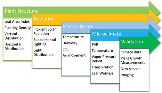
Figure 1. Researchers are taking a step-wise progression to modeling, first beginning with plant structure and moving towards validation. Image Credit: AAFC
Energy and mass balance
Greenhouse climate control focuses on achieving a steady-state relationship – a balance. The amount of energy and mass entering the system is equal to the amount leaving the system, but at a specific setpoint that is best for the plant. In our case, energy enters as heat and light, and leaves as heat. Mass entering the system can be water uptake through the roots, humidity through fans/vents under poor control, misting systems, for instance, though most models do not account for the water and sugar assimilated by the plant because it is such a small percentage. Ideally, this balance is achieved with as little energy leaving the system as possible. This energy and mass balance follows well-defined physical relationships that can be calculated
The challenge arises due to the rate of change and variation across the greenhouse. Any change in the input variables, such as increased sunlight, leads to a change in this balance. Just as there is a balance between the greenhouse macroclimate and the outside climate, there is a balance between the plant microclimate and the greenhouse macroclimate, which is impacted by the same laws of physics. As mentioned, there is significant variation in the microclimate throughout the greenhouse: this leads to the flow of heat and water vapour in many directions at the same time, and all these flows are interrelated and influence each other. With all these interactions, how can we begin to solve any of the individual balances?
Crop architecture
To begin creating a solution, we first have to define how specific it needs to be. Do we simulate the balance across every single leaf, so that we can predict the exact amount of energy each plant is converting to biomass for us? Or can we just pretend that there is one great big leaf in the middle of the greenhouse, equal to the area of all the leaves put together?
There are advantages and disadvantages to either approach. While modeling every single leaf would provide the most accuracy, a single simulation run through this model would likely take years to finish a single prediction, if it were even possible to define the location of every single leaf. With only one balance calculation required, the second option of simulating one great big leaf would certainly be faster, but we know that the climate can vary significantly across a greenhouse so the “average” we predict might be too general to be valid anywhere.
At Harrow, we have the benefit of possessing large historical datasets, containing plant growth measurements across entire growing seasons. These measurements include leaf dimensions and light distribution, both between rows, and vertically within the canopy. By feeding all this data into a computer, we can create what’s known as a density function, a mathematical formula that provides a probability of a leaf being in a specific area of the greenhouse as a function of time.
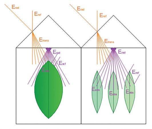
Figure 2. Big leaf model (left) and density function approach (right). Image credit: AAFC
Looking to Figure 2, we use a combination of two approaches. The opaque “big leaf” model on the left represents separate rows, while the translucent “medium leaves” on the right, represent the leaf distribution within each row. The graphics simply represent the probability of there being a leaf at a given height in the canopy. Each of these leaf density estimations can represent a row and a height in the greenhouse crop, or in modeling terms, a “node” of the model. Instead of assuming that the node intercepts all the light that hits it, we can treat each node as a filter that lets through some light to the nodes below it based on the leaf density function, with each node receiving less light than the ones above. Because we can’t yet reliably measure where we would find leaves in the canopy, instead of trying to guess where real opaque leaves would be, we treat each node as a location containing a large translucent leaf. If, from measurement, we know that there is a 30 per cent chance of a leaf being in a particular spot, we treat the translucent leaf as a filter that blocks 30 per cent of the light, and allows 70 per cent through to lower layers. Once we know how much light reaches each layer, the remaining microclimate variables can be calculated. Of course, no model is perfect, and the tradeoff with this approach is less accurate simulation of air movement in the canopy
Validation: sensors, imaging, and limitations
One of the major challenges of mathematical modeling is interpreting the results. The output will be large datasets full of temperature, vapour pressure deficit, transpiration, and light values at each node of the model. In addition to interpretation, it is also essential to ensure that the model is producing accurate results. Previous work at Harrow has developed microclimate monitoring towers, consisting of temperature, humidity and radiation sensors located at each modeled node to monitor the plant microclimate.
With the addition of LED lights to the greenhouse, we also need to consider the spectrum of light, not just the quantity, reaching each node. The spectrum can significantly impact crop development, and certain spectra of light are more likely to reach the bottom of the canopy. Future monitoring towers will need to be equipped for measuring spectrum to develop a more complete understanding of the greenhouse microclimate.
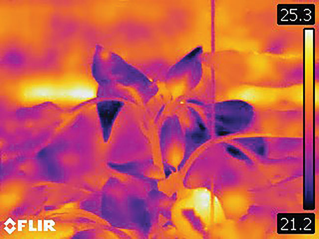
Figure 3. Thermal images of pepper plants under HPS (left) and LED (right). Image credit: AAFC
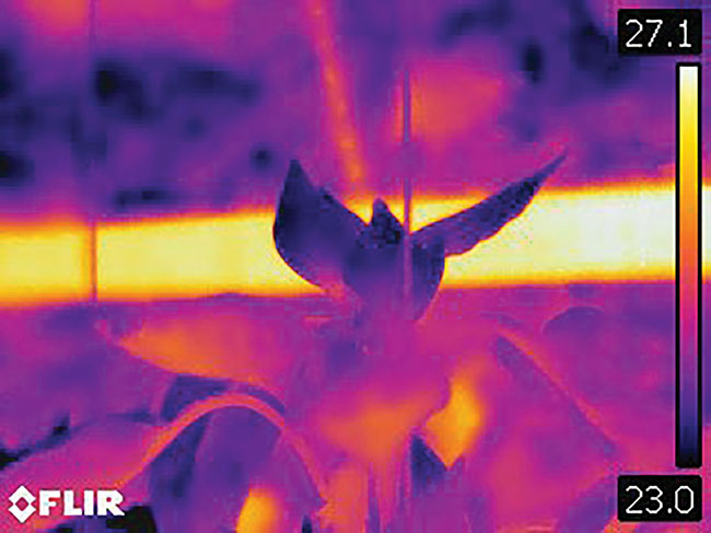
Different light sources also produce different amounts and types of heat. HPS lights produce more radiant heat, which directly warms up the crop canopy, whereas LED lights produce more convective heat, which is mixed with the greenhouse air. The effects on the microclimate can be directly observed with the use of an infrared camera. Figure 3 shows the growing head of a pepper plant under HPS on the left, and under LED light on the right. Both plants were grown in identical greenhouse compartments, maintained at identical climate control settings. Only the type of lighting was varied between the two pictures. The growing head under HPS varies from 21°C at the leaf tip, to 25°C at the stem, while the growing head under LED is a uniform 23°C. The crop under HPS light will have a warmer, drier microclimate at the same setpoint, but also have an increased rate of transpiration, shown by the cool leaf tip. The increased amount of water vapour exiting the plant causes a local cooling effect, as the evaporation of water requires a significant amount of energy absorbed from the surrounding area in the form of heat. While the drier climate with increased transpiration may lead to faster growth, it may also lead to increased stress, chlorosis, or vulnerability to disease.
So the question is, how do we find the correct balancing point for all these climate variables that would lead to faster crop growth without causing undue stress to the plant? The exact answer isn’t yet known, and leads to a limitation of microclimate modeling and measurement. Part of the challenge is that it varies significantly from greenhouse to greenhouse and crop to crop, especially with different light sources. While these models and datasets can be tremendously valuable, without the input, expertise, and observations from growers and researchers, the model results are just a large matrix of numbers. The continued optimization of greenhouse climate control will take coordinated efforts from researchers, growers, modelers, and control engineers to fully solve the complex puzzle before us.
Quade Digweed is a greenhouse engineer at Agriculture and Agri-Food Canada (AAFC). He can be reached at quade.digweed@canada.ca.
Print this page